Dashboarding made easy using Python and Elasticsearch
Building powerful dashboards using python, elasticsearch, apache Kafka and Kibana
Stream processing is an extremely powerful data processing paradigm which helps us process massive amounts of data points and records in the form of a continuous stream and allows us to achieve real time processing speeds.
Apache Kafka is an extremely powerful tool when it comes to data streams. It is highly scalable and reliable. [1]
Elasticsearch is a search engine based on the leucine library. It provides a distributed, full text search engine with an HTTP web interface and schema-free JSON documents. [2]
Kibana is an excellent tool for visualising the contents of our elasticsearch database/index. It helps us in building dashboards very quickly. [3]
Python is everybody’s favourite language because it is very easy to use.
In this blog, we will see how we can leverage the power of the stack above and create a dashboard from real data.
In order to simulate a streaming data source we will be using a log file containing random system logs and we will be pushing this information to a kafka topic. The architecture of the entire system is given below in Fig 1

Let’s start off with our kafka producer code. Let’s call this Producer.py. In this file we will do the following → Load the contents of the log file and parse it, push the data to a kafka topic for it to be consumed by our other python program which will be pushing this information to elasticsearch. The Kafka producer code block is shown in the code snippet below (Fig 2). A producer object is created in the constructor call. The produce method takes a message, converts it into a json and pushes it to the kafka topic specified

For this program I am using the confluent_kafka python package. Github link → https://github.com/confluentinc/confluent-kafka-python
Let’s have a look at our log file before writing a parser for it. Fig 3 below shows some lines from the log file.

The code block (Fig 4) which parses the log and returns message in a python dictionary format is given below. While examining the log file we noticed that the log messages are of the following types → [“INFO”, “ERROR”, “CRITICAL”, “WARNING”] . This information will be helpful during categorising our data on the Kibana dashboard.

The parser class in Fig 4 is fairly straight forward. We have a couple of functions to load the log file and return each row using an iter function.
Once we have our log file parser and kafka producer in place, we can go ahead and send the log messages to our kafka topic. These messages will then be picked up by a consumer and pushed to elasticsearch. Fig 5 shows how we are calling the methods to push messages into the kafka topic.

On running the main function, the contents of the log file get pushed to the kafka topic and received by the consumer on the other end. The output is given below in Fig 6.

Next, we will go ahead and code the section for pushing all this information onto Elasticsearch and then move forward with the dashboard creation on Kibana.
For connecting to Elasticsearch with python we will be using the official Elasticsearch library for python→ https://elasticsearch-py.readthedocs.io/en/v7.13.0/
In Fig 7, we have the class called Elastic where we connect to our elasticsearch instance running on port 9200. For this experiment we are using a docker-compose file containing the config for both the elasticsearch and kibana services. The docker-compose file is present in the GitHub repo for this experiment (link at the end of the blog). A simple docker-compose up should start our elasticsearch and kibana instances.

The data structure that Elasticsearch uses to store data is called an inverted index. It has the capability of uniquely identifying every word very fast. As a result, we are able to execute searches and queries at real-time speeds. In our experiment, the name of the index is “new-relic-log”
The Kafka consumer block is given in Fig 8 which we will be using for reading messages from the kafka topic to which the producer was sending all the log messages. The read_messages method lets us constantly poll the topic and look for messages.

Once we have the messages coming in from the consumer, we can call the push_to_index method in the Elastic class to push the message to Elasticsearch as shown below in Fig 9

The output of the commands in Fig 9 is shown in Fig 10 below. The write response shows the detail of our data transfer to elasticsearch with index details and also the result.

Now let’s see how the data shows up on Elasticsearch. In order to access our index we will directly move to our Kibana dashboard. Make sure that your Kibana and Elasticsearch containers are running properly. Head over to http://localhost:5601 ← This is the port on which Kibana is running on my local machine. The home screen for Kibana is shown in Fig 11 below

Now to check if the data is properly coming to our new-relic-log index, click on the Discover button (second button on the panel on the left hand side), as shown in Fig 12. Select the index as new-relic-log from the drop-down menu and you should see all the log messages sent by python getting populated on the centre of the screen (Fig 13)


In order to filter out just the INFO logs or the ERROR logs, we can use the search bar on the top, which provides us with many options to filter out our data points. An example of the INFO logs being filtered out is shown in Fig 14 below

Now in order to visualise our data and put it on a real dashboard, we will have to prepare some charts. Let’s go ahead and start of with a line chart. This line chart will aggregate the count of the different log types and display it.
Click on the Visualise button, right below the Discover button on the panel on the left side (Fig 15).

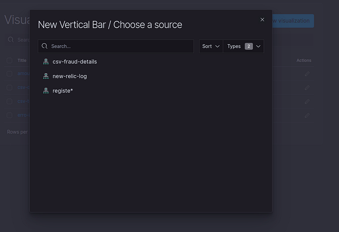
As soon as you click on the Create new visualization button, you will be presented with quite a few different types chart options (Fig 16). For this example, we will be using the line chart

Once you have chosen your preferred chart type, you will be prompted with the choice of index to read the data from. Here, we will be choosing the new-relic-log index (Fig 17)
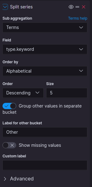
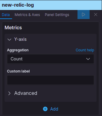
Now, we will be creating the settings for our line chart. On the Y-axis we will choose the parameter as Count. On the X-axis we will be choosing the parameter as timestamp. Kibana also provides us with an option to split the chart over the same X-axis between different keys. In our case, we will be visualizing the count of INFO logs and ERROR logs on the same chart. The settings are shown in Fig 18(a,b) and 19 respectively. The final chart is shown in Fig 20. As you can see, we have the aggregation over the timestamps for both the log types.


We have also created a pie-chart to get a total count of the two different log-types (Fig 21). In order to create the pie-chart, just choose the pie-chart option on the visualization screen instead of the line-chart option.

Now we will be creating our first Kibana dashboard. This step cannot get any simpler.
Click on the Dashboard button just below the Visualize button. Click on the add button on top → Choose the chart and done. You have your dashboard ready (Fig 22)

I hope this blog was helpful in giving a brief walk-through of how we can leverage the power of these open source tools to build robust data streaming pipelines.
Github link to the project →https://github.com/AbhishekBose/kafka-es
References:

